How honest is one sample per month? A spectral audit
Part 3 of a three-part series on computing the El Niño index with SQL over cloud-hosted array data: Part 1 — reproducing NOAA’s official index from ERSST · Part 2 — the independent ERA5 cross-check · Part 3 (this post).
Across Part 1 and Part 2 we flagged one deliberate shortcut: the ERA5 recipe builds each “monthly” sea-surface temperature from a single hourly field — 12:00 UTC on the 15th — rather than averaging all ~720 hourly steps in the month. It keeps the remote reads cheap. But is it honest? A single mid-month snapshot could inject weather-scale noise that a true monthly mean would smooth away.
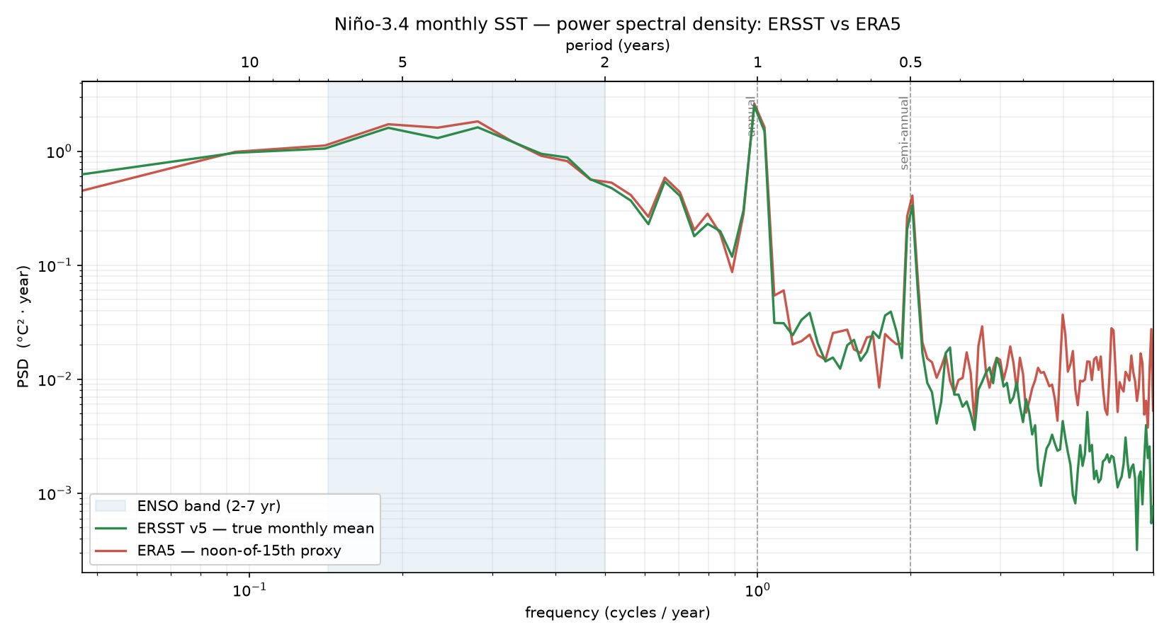
This post measures the damage. The verdict: the shortcut adds excess power only in the high-frequency band the ONI never listens to, and preserves the low-frequency ENSO variance almost exactly. It’s a cheap approximation that happens to be cheap in the right place.
The idea: use a true monthly mean as the ruler
We don’t have to guess how much the snapshot distorts the signal — we have a genuine monthly-mean SST record for the same box: ERSST v5, the dataset from Part 1. ERSST is a true monthly average by construction. So it’s the perfect ruler: line the ERA5 snapshot series up against the ERSST monthly series over the Niño-3.4 box, and any spectral difference is the fingerprint of the sampling choice.
Both series come from one SQL join — ERSST read in place via VirtualiZarr, ERA5 from ARCO-ERA5, paired month by month:
SELECT
  make_date(e.yr, e.mo, 1) AS time,
  ROUND(e.sst_c, 4)        AS sst_ersst,   -- true monthly mean
  ROUND(a.sst_c, 4)        AS sst_era5     -- day-15 / noon-12 snapshot
FROM ersst_monthly e
JOIN era5_monthly  a ON a.yr = e.yr AND a.mo = e.mo
ORDER BY e.yr, e.mo;
(The full query — both _monthly CTEs — is nino34_monthly_sst.sql.)
The method: split the variance by timescale
Once we have the paired series, we compare their power spectral densities — how each series distributes its variance across timescales — with a standard Welch estimate:
- sampling rate 12 samples/year, segments of 256 months (~21 years), Hann window, density scaling;
- linear detrend first, so the mean and the warming trend don’t dominate the low-frequency end;
- then integrate the power in three bands and take the ERA5/ERSST ratio in each:
- ENSO band — 2 to 7 years (0.143–0.5 cycles/year): this is what the ONI measures
- Annual cycle — 0.9–1.1 cycles/year
- High-frequency / noise — above 1.5 cycles/year: sub-8-month wiggles
If the snapshot were corrupting the ENSO signal, we’d see excess ERA5 power in the first band. If it’s only adding weather-scale noise, the excess shows up in the third.
The result: noise where it doesn’t matter
The excess power from the snapshot is confined to the high-frequency regime:
| Band | Timescale | ERA5 / ERSST power |
|---|---|---|
| ENSO | 2–7 years | ≈ 1 (variance preserved) |
| Annual | ~1 year | ≈ 1 |
| High-frequency | < 8 months | ~1.64× |
The ENSO band — the only part the 3-month-averaged ONI actually integrates — is preserved. The one-sample-per-month choice adds roughly 1.64× excess power at high frequencies, exactly where you’d expect a single mid-month snapshot to carry weather that a full average would cancel. And crucially, the ONI’s own 3-month running mean is itself a low-pass filter: it attenuates precisely the high-frequency band where the excess lives.
So the shortcut is honest in the way that matters. It’s noisy — but noisy in a band the index discards, and quiet in the band the index sums. That’s why Part 2’s residuals scatter a little month-to-month yet never once flip an ENSO sign.
The road not taken
The faithful alternative is to average all ~720 hourly steps per month instead of sampling one. That’s not a harder query — it’s a bigger read: every hourly field for the whole box, back to 1940, is orders of magnitude more remote I/O than one timestep per month. Done naively it turns a 60-second in-region query into a heavy scan. The honest way to ship it is a distributed-execution variant that fans the hourly reduction across workers — which we’ve deferred until the infrastructure to run it cheaply is in place.
Until then, this audit is the justification for the shortcut: we measured what it costs, found the cost lands in a band the ONI ignores, and kept the cheap path with eyes open.
The series, in one line
- Part 1 — reproduce NOAA’s official ONI from ERSST, in place over NetCDF, to 0.001 °C.
- Part 2 — confirm it independently from ERA5: 0.16 °C, r = 0.966, zero sign reversals.
- Part 3 (this post) — show the one shortcut in Part 2 is honest, using Part 1’s ERSST as the ruler.
Three posts, two datasets, one methodology — and never once a downloaded copy.
Run it yourself
The el-nino-oni cookbook has the paired-series query, the spectral comparison script (psd_compare.py), and the plot. If you’re weighing a cheap sampling shortcut against a full aggregation in your own array pipelines and want to know what it actually costs you, that’s the kind of question SQL-in-place makes easy to answer — reach us at [email protected].
References
- zarr-datafusion — SQL engine for Zarr-native (and, via VirtualiZarr, NetCDF) array data
nino34_monthly_sst.sql·psd_compare.py- Part 1 — ERSST exact reproduction · Part 2 — ERA5 cross-check